Map Development
If you’ve read through the main tutorial then you can skip this, but here’s a quick, non-exhaustive, note on terminology related to the game map:
- Tiles
-
The core foundation of the map. These are the chunks of land that players move their armies on and fight directly over. Tiles which border seas are considered “Coastal.” You can build buildings and—if the tile contains a center—units, on them
- Seas
-
Like tiles, players move their navies on and fight over these. Notably, seas differ in that they do no contain centers, nor do they constitute provinces or regions, nor even can anything be built on them (you can’t build a building or units in a sea, you can only move in navies). These are pure battlegrounds. If a tile is entirely surrounded by a sea (think of a small island), that tile is considered to “belong” to the sea, meaning that the pair of areas is considered to act as a single area.
e.g., a navy controlling the sea also controls the island, nothing can be put on the island. This is to avoid some seas with small islands becoming near-impenetrable as players could otherwise stack units in each island to defend the navy.
- Centers
-
Exclusively present on some tiles, these are represented by small circles on tiles where they are present. They earn income and action points for the players who control them, and allow players to build units if the player can support them.
- Provinces
-
Constituted by a group tiles, and owned by a player if that player controls all centers within the province.
e.g., if a province is made up of 5 tiles, and 3 of those tiles have centers, then you must control at least the 3 tiles with centers to control the province). These earn bonuses to income and action points for players who control them.
- Regions
-
Constituted by a group of provinces, and owned by a player if that player controls all provinces within the region.
- Buildings
-
Can only be built on tiles. There are two buildings:
Forts: Add +1 defense to the tile where they are built;
Supply Hubs: Allow units adjacent to the supply hub to move two tiles in one move order (typically they can only move one) where possible:
e.g., if there is an empty tile (or sea!) in front of a unit, and that unit is adjacent to a supply hub (either in the same tile or one next to the unit), then that unit can move through that empty tile and execute an order in the next ones adjacent to the empty tile. This only works if the intermediate tile in the order is empty! You cannot phase through an enemy to attack behind their lines.
and allow for units to be built as if the tile was a center.
Overview
This page details how the game map is created: how the data is generated, displayed, and interacted with. Code chunks are partly supplied for demonstration, although for full and functional code, please go to the game repo.
To be brief: Chicanery uses .Rds files to store and manage game data. One such file (gamedata.Rds) contains all map data, including:
- Tiles, and seas, and their geometry;
- To what province each tile belongs;
- To what region each province belongs;
- Whether the tile is coast, and/or if the tile “belongs” to a sea;
- Whether the tile contains a center, a fort, and/or a supply hub.
This is helpful in keeping the game realtively lightweight, and works well with R. To create this dataset, we first draw our map by layer (Tiles, Seas, Provinces, etc.) using unique-valued RGB colors for each shape, and export each layer individually as a .png file. You can do this however you like: using Adobe Photoshop, GNU Image Manipulation Program, or some other editor. We then feed these files into a script, mapDataGenerate.R, that scrounges each pixel of each file and groups them by RGB value. The result is a list of tile and sea geometries: polygons and multipolygons, and their adjacencies. We then assign tiles to their respective provinces and regions by checking which province and region geometries the centroids of each tile fall into and do the same to assign centers, and assign tiles adjacent to seas as coastal. Lastly, we manually define which tiles are occupied to begin with, and what units—if any—occupy them. With this done, we have our complete dataset.
With the dataset, we export “blank” layers for the tiles, provinces, and regions, to serve as backgrounds for the map in-game, and use ggplot2 and ggiraph to create an interactive map using the data. For a semi-step-by-step guide on how the base map for the game was created (including parts that aren’t required for new map generation in general), check the sections below.
Creating the Base Map
The map in the base game is similar to that of standard-variant Diplomacy. To recreate it with relative precision, a little style, and not too much tracing, we can plot out the real map, import that into an image editor to edit our layers, and run the output through the mapDataGenerate.R script.
An Outline to Start
To begin we can use R to generate a large, border-less, map of European and North African provinces:
library(dplyr)
library(ggplot2)
library(rnaturalearth)
library(rmapshaper)
library(sf)
# This is a border outline for manual later use where needed; it is *not* used for map-gen.
top_level_tiles <- ne_countries(scale = 50, returnclass = "sf") %>%
ms_simplify(keep = 0.1, keep_shapes = TRUE) %>%
ggplot() + geom_sf(lwd = 0.25, color = "white", fill = "transparent") +
coord_sf(crs = st_crs(3035),
xlim = c(1800000, 6800000),
ylim = c(1000000, 6000000)) +
theme_void() +
theme(
legend.position = "none"
)
ggsave(plot = top_level_tiles, filename = "map_data/top_level_tiles.tiff", width = 4, height = 2.25, device='tiff', dpi=960)
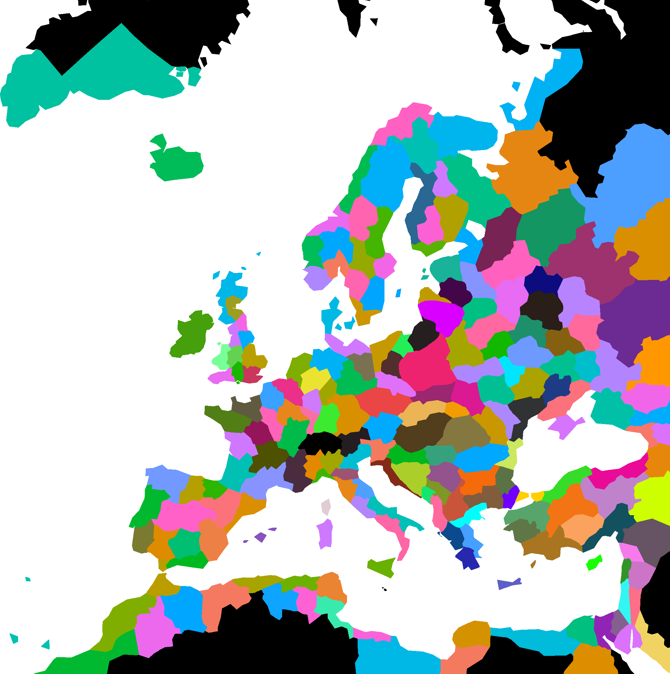
tiles <- ne_states(country = c("Iceland", "Ireland", "United Kingdom", "Norway", "Sweden", "Finland", "Russia", "Denmark", "Estonia", "Latvia", "Lithuania", "France", "Luxembourg", "Belgium", "Netherlands", "Germany", "Czech Republic", "Poland", "Belarus", "Switzerland", "Austria", "Slovakia", "Ukraine", "Portugal", "Spain", "Andorra", "Monaco", "Italy", "Vatican City", "San Marino", "Slovenia", "Hungary", "Croatia", "Bosnia and Herzegovina", "Serbia", "Romania", "Moldova", "Montenegro", "Republic of Serbia", "Kosovo", "Albania", "Macedonia", "Bulgaria", "Greece", "Turkey", "Morocco", "Algeria", "Tunisia", "Cyprus", "Libya", "Egypt", "Israel", "West Bank", "Lebanon", "Syria", "Jordan", "Iraq", "Armenia", "Georgia", "Azerbaijan", "Saudi Arabia", "Kuwait", "Iran", "Kazakhstan", "Northern Cyprus", "Malta", "Greenland"),
returnclass = "sf") %>%
ms_simplify(keep = 0.01, keep_shapes = TRUE) %>%
ggplot() + geom_sf(aes(fill = name), lwd = 0) +
coord_sf(crs = st_crs(3035),
xlim = c(1800000, 6800000),
ylim = c(1000000, 6000000)) +
theme_void() +
theme(
legend.position = "none"
)
tiles
ggsave(plot = tiles, filename = "map_data/tiles.tiff", , width = 4, height = 2.25, device='tiff', dpi=960)Now we have a good foundation! Take this and put it into an image editor.
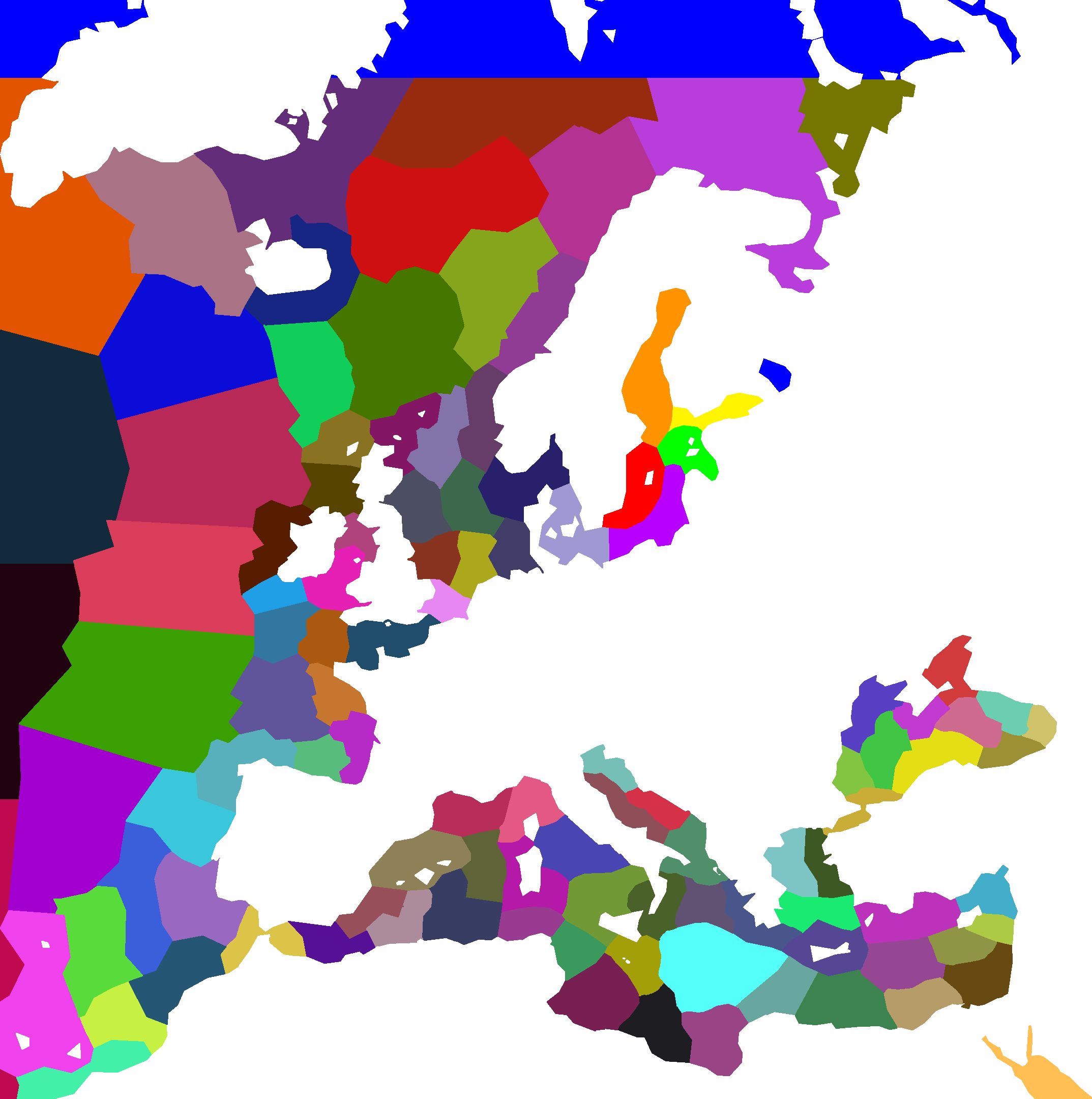
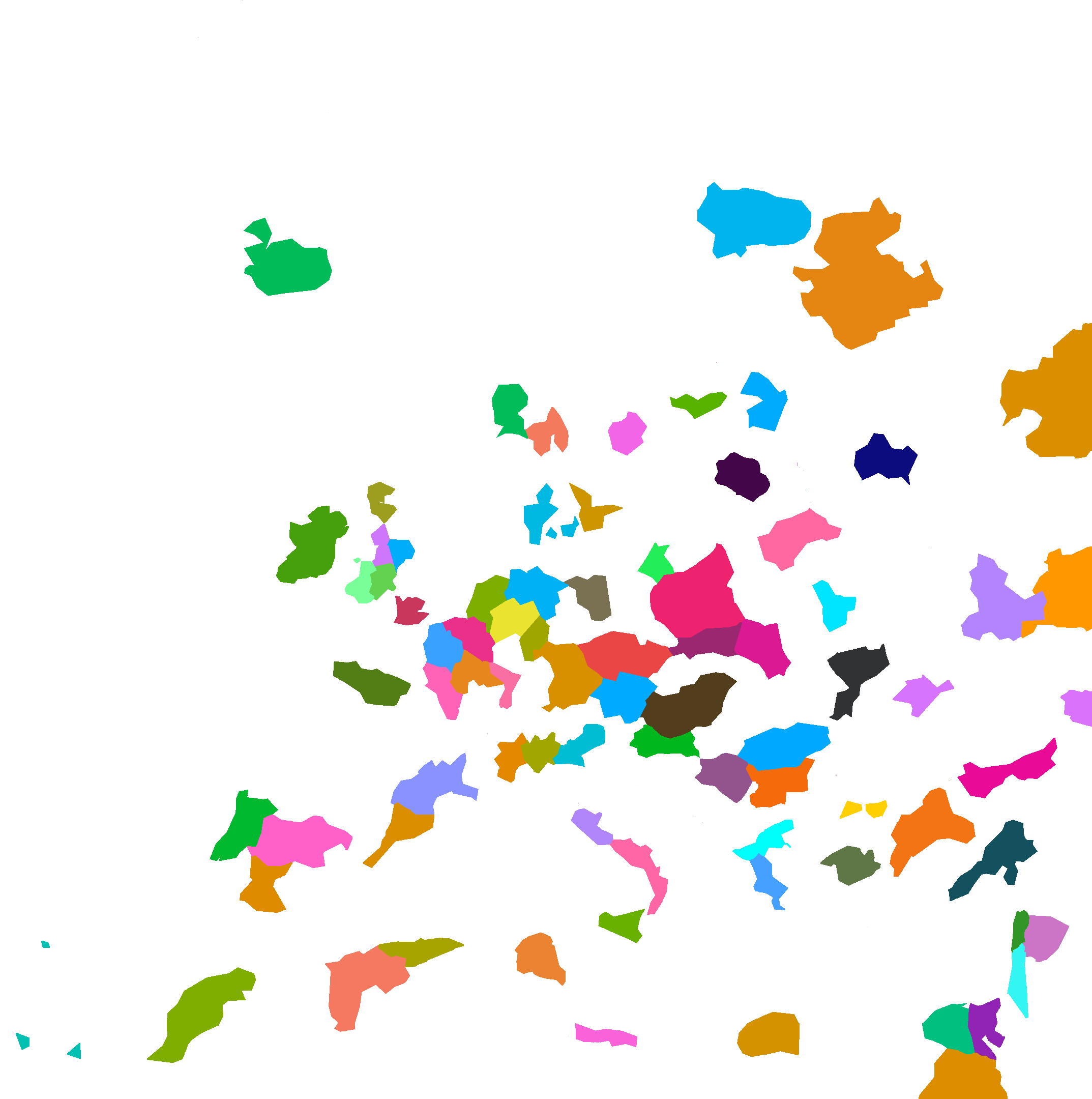
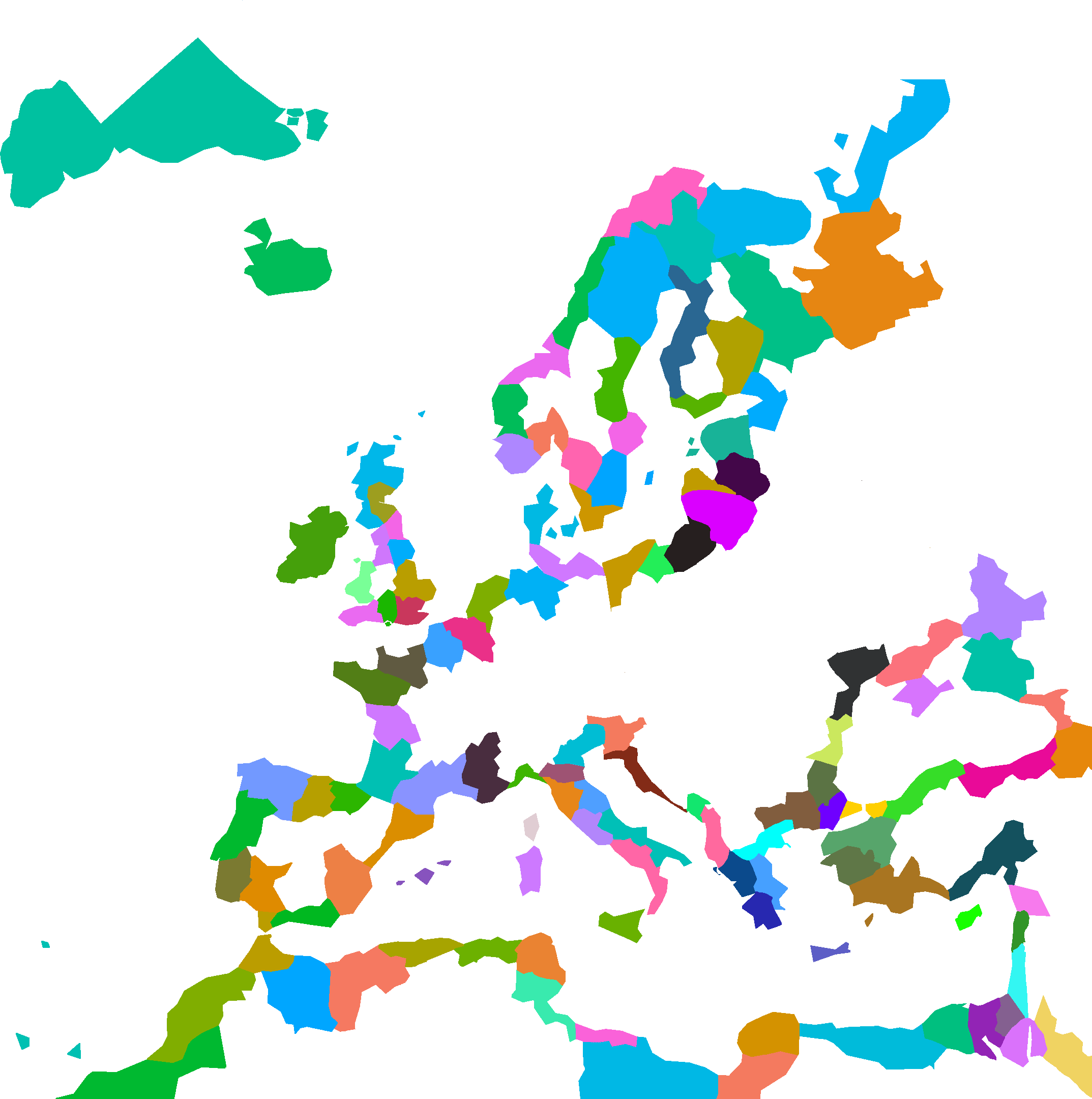
Taking Form
Taking that map, we import it into GNU Image Manipulation Program across six layers:
and edit to our hearts’ desire. Remember to assign unique RGB values to each shape in each layer! This process can be very long, but doesn’t require much technical explanation—just draw how you want things to look. When done, export each layer as an 8-bit RGBA .png file. This is our result:
Read the Script
With our files ready, we run mapDataGenerate.R. We begin by first reading in our .png files:
library(dplyr)
library(ggplot2)
library(geojsonsf)
library(nngeo)
library(plotly)
library(png)
library(sf)
library(smoothr)
library(tidyr)
library(tidyverse)
library(jsonlite)

# Load raw map image files
regions <- readPNG("data/raw/REGIONS.png")
provinces <- readPNG("data/raw/PROVINCES.png")
tiles <- readPNG("data/raw/TILES.png")
seas <- readPNG("data/raw/SEAS.png")
coasts <- readPNG("data/raw/COASTS.png")
centers <- readPNG("data/raw/CENTERS.png")
These just store the images in large list array formats. If you want, you can do plot(tiles), or some other layer, to see the image in the R viewer. We then take each of these images, and run them through a function we’ve made, unravelCoords():
regionData <- unravelCoords(regions, "REGION") %>%
  st_as_sf()
provinceData <- unravelCoords(provinces, "PROVINCE") %>%
  st_as_sf()
tileData <- unravelCoords(tiles, "TILE") %>%
  st_as_sf()

# ... etc, etc.
This function is comprised of a good little chunk of code and some helper functions all cobbled together, but in practice what it does is: check the dimensions of an image, and map each pixel to a coordinate within the dimensions while recording the RGB value of the pixel, then finally grouping pixels with alike RGB values together and spitting out the coordinates to re-draw the shape those pixels made. After this process is done, we combine seaData and tileData into a set called gameMapShapes and use information from the other sets to inform some additional columns and work. Please check the file of reference, mapDataGenerate.R, if you want to go in depth on these processes. Lastly, we figure out which tile is where:
labels_test <- ggplot(gameMapShapes) + geom_sf() + geom_sf_text(aes(label = shape), size = 0.5)
and manually assign some tiles to be owned by certain countries at the start of the game:
gameMapShapes <- gameMapShapes %>%
  mutate(occupied_by = case_when(
    ### GBR: 6 (Notice how it holds 2 non-centers at start... stretched thin!)
    shape == "TILE_139" ~ "GBR", #center
    shape == "TILE_87" ~ "GBR", #center
    shape == "TILE_148" ~ "GBR", #center
    shape == "TILE_116" ~ "GBR", #center
    shape == "TILE_134" ~ "GBR",
    shape == "TILE_29" ~ "GBR", #center
    shape == "TILE_160" ~ "GBR", #center
    shape == "TILE_49" ~ "GBR",
    ### FRA: 5
    shape == "TILE_80" ~ "FRA", # center
    shape == "TILE_205" ~ "FRA", # center
    shape == "TILE_169" ~ "FRA", # center
    shape == "TILE_101" ~ "FRA", # center
    shape == "TILE_121" ~ "FRA", # center
    ### GER: 6 (same count as britain, but all in one place)
    shape == "TILE_194" ~ "GER", #center
    shape == "TILE_97" ~ "GER", #center
    shape == "TILE_54" ~ "GER", #center
    shape == "TILE_161" ~ "GER", #center
    shape == "TILE_10" ~ "GER", #center
    shape == "TILE_118" ~ "GER", #center
    ### RUS: 7
    shape == "TILE_165" ~ "RUS", #center
    shape == "TILE_6" ~ "RUS", #center
    shape == "TILE_152" ~ "RUS", #center
    shape == "TILE_43" ~ "RUS", #center
    shape == "TILE_212" ~ "RUS", #center
    shape == "TILE_40" ~ "RUS", #center
    shape == "TILE_209" ~ "RUS", #center
    ### AHE: 4
    shape == "TILE_5" ~ "AHE", #center
    shape == "TILE_188" ~ "AHE", #center
    shape == "TILE_79" ~ "AHE", #center
    shape == "TILE_14" ~ "AHE", #center
    ### ITA: 4 (spread between europe and north africa like a mini-france)
    shape == "TILE_195" ~ "ITA", #center
    shape == "TILE_130" ~ "ITA", #center
    shape == "TILE_26" ~ "ITA", #center
    shape == "TILE_164" ~ "ITA", #center
    ### OTT
    shape == "TILE_213" ~ "OTT", #center
    shape == "TILE_183" ~ "OTT", #center
    shape == "TILE_142" ~ "OTT", #center
    shape == "TILE_170" ~ "OTT", #center
    shape == "TILE_48" ~ "OTT", #center
    TRUE ~ "unoccupied"
  ))
With that done, we at last check for and add adjencencies:
adj_nested_list <- list()
for (i in 1:nrow(gameMapShapes)) {
  temp_adj_i_list <- list()
  for (j in 1:length(as.list(strsplit(gsub("\n","", gsub(" ", "", gsub("\"", "",gsub("[c()]", "", (gameMapShapes$adjacency_list[i]))))), ",")[[1]]))) {
    temp_adj_i_list[[j]] <-  toString(as.list(strsplit(gsub("\n","", gsub(" ", "", gsub("\"", "",gsub("[c()]", "", (gameMapShapes$adjacency_list[i]))))), ",")[[1]])[j])
  }
  adj_nested_list[[i]]  <- temp_adj_i_list
}

gameMapData <- gameMapData_no_adj
gameMapData[["adj"]] <- adj_nested_list
at last arriving at our conclusion for map generation:
 :::{.callout-note collapse=“true”} ## Plot Code
map_plot <- ggplot() +
  geom_sf(data = gameMapShapes, color = "white") +
  geom_sf(data = (gameMapShapes %>% filter(substr(tile, 1,3) == "SEA")), fill = "blue") +
  geom_sf(data = (gameMapShapes %>% filter(occupied_by == "unoccupied") %>% filter(!is.na(ofRegion))), fill = "beige") +
  geom_sf(data = (gameMapShapes %>% filter(occupied_by != "unoccupied")), aes(fill = occupied_by)) +
  geom_sf(data = st_as_sf(as.data.frame(gameMapShapes) %>% filter(center == TRUE) %>% select(centroid)), color = "black", size = 1.5) +
  geom_sf(data = st_as_sf(as.data.frame(gameMapShapes) %>% filter(center == TRUE) %>% select(centroid)), color = "white", size = 1) +
  geom_sf_text(data = (gameMapShapes %>% filter(unit != "none")), aes(label = unit), size = 2) +
  scale_fill_brewer(palette = "Dark2", direction = 1) +
  theme_void() +
  theme(
    legend.position = "bottom"
  ) +
  labs(
    fill = "Country"
  )
ggsave("data/extras/map.png", map_plot, width = 16, height = 9)
:::
Now we export just the background layers for tiles, provinces and regions (with seas in each of course):

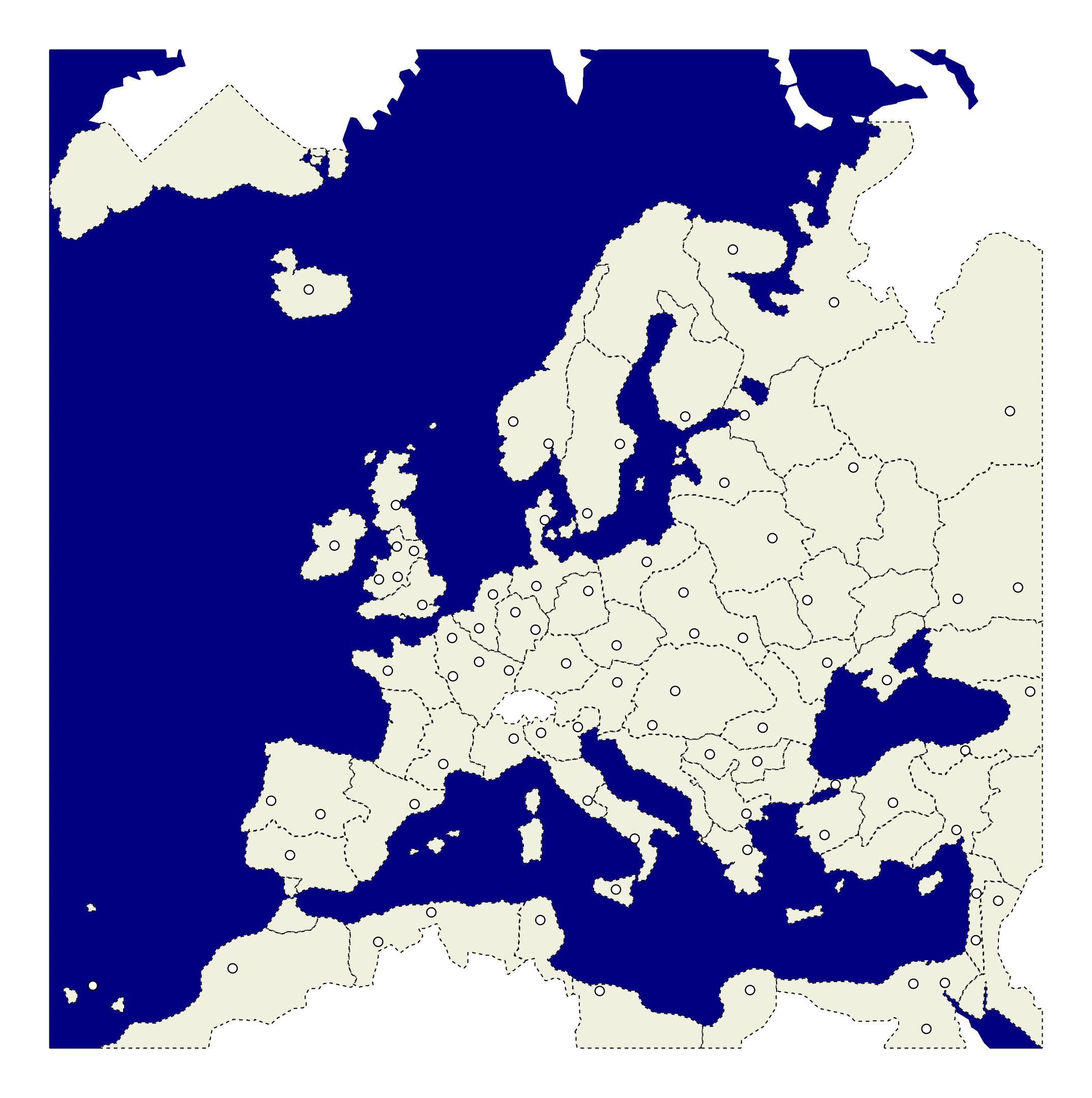

the code for those backgrounds is below:
tile_bg <- ggplot() +
  geom_sf(data = (map_data %>% filter(substr(tile, 1, 3) == "SEA")), fill = "navy", color = "navy") +
  geom_sf(data = (map_data %>% filter(substr(tile, 1, 4) == "TILE")), fill = "beige", color = "beige") +
  geom_sf(data = (map_data %>% filter(substr(tile, 1, 4) == "TILE")), color = "black", linetype = "dashed", alpha = 0.3) +
  geom_sf(data = st_as_sf(as.data.frame(map_data) %>% filter(center == TRUE) %>% select(centroid)), color = "black", size = 1.5) +
  geom_sf(data = st_as_sf(as.data.frame(map_data) %>% filter(center == TRUE) %>% select(centroid)), color = "white", size = 1) +
  theme_void() +
  theme(
    legend.position = "none",
    axis.line = element_blank(),
    panel.grid.major = element_blank(),
    panel.grid.minor = element_blank(),
    panel.border = element_blank(),
    panel.background = element_blank(),
  )
ggsave(tile_bg, filename = "data/map/tilemap.png", width = 2147, height = 2160, units = "px", dpi = 320)
province_bg <- ggplot() +
geom_sf(data = (map_data %>% filter(substr(tile, 1, 3) == "SEA")), fill = "navy", color = "navy") +
geom_sf(data = (map_data %>% filter(substr(tile, 1, 4) == "TILE")), fill = "beige", color = "beige") +
geom_sf(data = (map_data %>% filter(substr(tile, 1, 4) == "TILE") %>% group_by(ofProvince) %>% summarize(geometry = st_union(geometry)) %>% st_remove_holes()), color = "black", linetype = "dashed", alpha = 0.3) +
geom_sf(data = st_as_sf(as.data.frame(map_data) %>% filter(center == TRUE) %>% select(centroid)), color = "black", size = 1.5) +
geom_sf(data = st_as_sf(as.data.frame(map_data) %>% filter(center == TRUE) %>% select(centroid)), color = "white", size = 1) +
theme_void() +
theme(
legend.position = "none",
axis.line = element_blank(),
panel.grid.major = element_blank(),
panel.grid.minor = element_blank(),
panel.border = element_blank(),
panel.background = element_blank(),
)
ggsave(province_bg, filename = "data/map/provincemap.png", width = 2147, height = 2160, units = "px", dpi = 320)region_bg <- ggplot() +
geom_sf(data = (map_data %>% filter(substr(tile, 1, 3) == "SEA")), fill = "navy", color = "navy") +
geom_sf(data = (map_data %>% filter(substr(tile, 1, 4) == "TILE")), fill = "beige", color = "beige") +
geom_sf(data = (map_data %>% filter(substr(tile, 1, 4) == "TILE") %>% group_by(ofRegion) %>% summarize(geometry = st_union(geometry)) %>% st_remove_holes()), color = "black", linetype = "dashed", alpha = 0.3) +
geom_sf(data = st_as_sf(as.data.frame(map_data) %>% filter(center == TRUE) %>% select(centroid)), color = "black", size = 1.5) +
geom_sf(data = st_as_sf(as.data.frame(map_data) %>% filter(center == TRUE) %>% select(centroid)), color = "white", size = 1) +
theme_void() +
theme(
legend.position = "none",
axis.line = element_blank(),
panel.grid.major = element_blank(),
panel.grid.minor = element_blank(),
panel.border = element_blank(),
panel.background = element_blank(),
)
ggsave(region_bg, filename = "data/map/regionmap.png", width = 2147, height = 2160, units = "px", dpi = 320)having background layers like this makes the map easier to manage once we start making it interactive.
Interactivity
This section assumes you already have your map, whether it is the one described above or another. It’s time to start clicking!